Vegetarian Restaurant and Income
Ming Gong
Income=read.csv("data\\Income.csv",stringsAsFactors=F)

Income<-Income %>%
  rename(
    county_fips = State...County.Name,
    county_id=County.ID,
    povertyrate=All.Ages.in.Poverty.Percent
    )

Res=read.csv("data\\Restaurant.csv", stringsAsFactors=F)

a =Res$cuisines
vege <- str_detect(a,"Vegetarian")
ResV <- cbind(vege,Res)

ResV$vege <- as.numeric(ResV$vege)
ResVV <- subset(ResV,vege==1)
ResVVV <- ResVV %>%
  dplyr::select(id,city,name,latitude, longitude,phones,paymentTypes,postalCode) %>%
  mutate(latitude=as.numeric(latitude), longitude=as.numeric(longitude)) %>%
  na.omit()

latlong2county <- function(pointsDF) {
    # Prepare SpatialPolygons object with one SpatialPolygon
    # per county
    counties <- map('county', fill=TRUE, col="transparent", plot=FALSE)
    IDs <- sapply(strsplit(counties$names, ":"), function(x) x[1])
    counties_sp <- map2SpatialPolygons(counties, IDs=IDs,
                     proj4string=CRS("+proj=longlat +datum=WGS84"))

    # Convert pointsDF to a SpatialPoints object
    pointsSP <- SpatialPoints(pointsDF,
                    proj4string=CRS("+proj=longlat +datum=WGS84"))

    # Use 'over' to get _indices_ of the Polygons object containing each point
    indices <- over(pointsSP, counties_sp)

    # Return the county names of the Polygons object containing each point
    countyNames <- sapply(counties_sp@polygons, function(x) x@ID)
    countyNames[indices]
}

# Test the function using points in Wisconsin and Oregon.
testPoints <- data.frame(x = ResVVV$longitude, y = ResVVV$latitude)

county_list<- latlong2county(testPoints)

county_list_data<-as.data.frame(county_list)
VRes<-cbind(ResVVV,county_list_data)
VRes<-VRes %>%
  na.omit
#unique(VRes$county_list)

county_name <- as.character(VRes$county_list)
# Remove all before and up to ",":
county_name2 <- gsub(".*,","",county_name)
data <- cbind(county_name2,VRes)
data$county_list <- NULL
#unique(data$county_name2)

Income=read.csv("data\\Income.csv",stringsAsFactors=F)

Income<-Income %>%
  rename(
    county_fips = State...County.Name,
    county_id=County.ID,
    povertyrate=All.Ages.in.Poverty.Percent
    )
Income$county_id=as.character(Income$county_id)
How is the distribution of vegetarian restaurants in New York State? Does poverty rate relate to that distribution? To dive into those questions, we combine two datasets (one contains NY restaurants from datafiniti and another comes from U.S.Income & Poverty rate dataset) together for visualization.
Plot income(poverty) map
counties_sf <- get_urbn_map("counties", sf = TRUE)
counties_sf<-counties_sf %>%
filter(state_name == "New York")


spatial_data <- left_join(counties_sf,
                          Income,
                         by=c("county_fips"="county_id"))

ggplot() +
  geom_sf(spatial_data,
          mapping = aes(fill = povertyrate),
          color = "#ffffff", size = 0.25) +
  labs(fill = "povertyrate")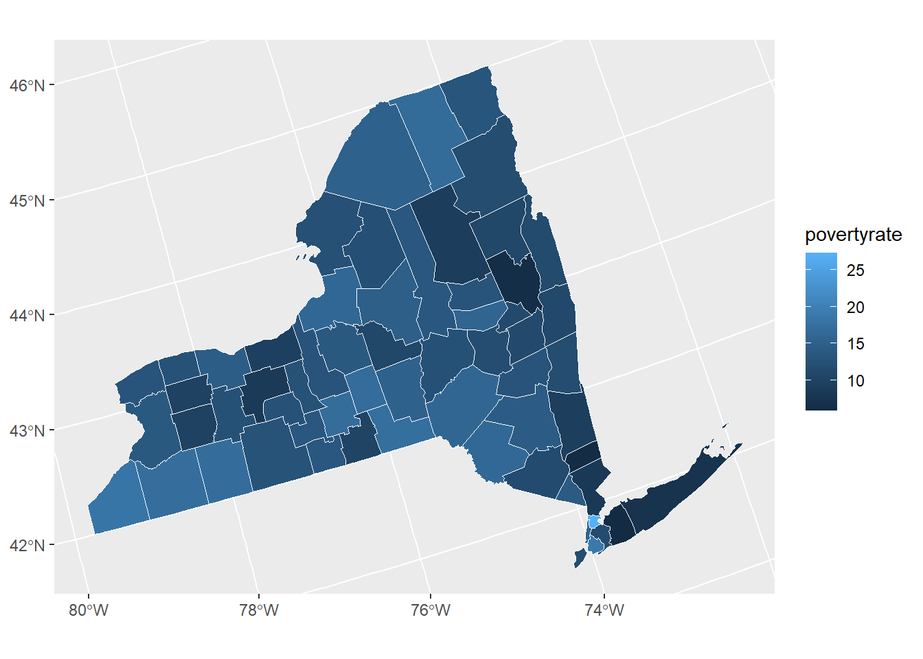
data1 <- st_as_sf(data, coords = c("longitude", "latitude"),
crs = 4326, agr = "constant")

g<-ggplot(data=spatial_data)+geom_sf(mapping = aes(fill = povertyrate))+geom_sf(data=data1,size = 4, shape = 23, fill = "darkred")+theme_map()+theme(legend.position="right")

g1<-ggplotly(g) %>%
  highlight(
    "plotly_hover",
    selected = attrs_selected(line = list(color = "black"))
)


g1
Data Visualization (QMSS Spring 2020) Group F: Vegan
Please do not hesitate to give us your feedback ❤
Source files and process book.